Load Packages & Set Preferences
library(tidymodels)
library(brulee)
library(modeldata)
library(tidyverse)
library(skimr)
tidymodels_prefer()
theme_set(theme_minimal())
set.seed(1234)Hyperparameter optimization is a key part of the machine learning workflow. Knowing what hyperparameters to choose or even which ones to change can be a bit overwhelming, especially when you have a lot of them. Iterative hyperparameter optimization is a common approach to this problem, but it can be time consuming and expensive. Bayesian optimization is a method that can help with this problem. For a deeper dive into Bayesian optimization and iterative optimization overall, Julia Silge and Max Kuhn’s Tidy Modeling with R has a great chapter on this topic.
In the whole game, I used Bayesian optimization for hyperparameterization but did not provide much explanation or justification. In this post, we’ll use Bayesian optimization to tune the hyperparameters of a neural net with {torch} and {brulee} using the tidymodels framework.
Silge and Kuhn’s share some advice with how to approach hyperparameter optimization and model screening in general:
A good strategy is to spend some initial effort trying a variety of modeling approaches, determine what works best, then invest additional time tweaking/optimizing a small set of models. Julia Silge and Max Kuhn, Tidy Modeling with R
Load Packages & Set Preferences
library(tidymodels)
library(brulee)
library(modeldata)
library(tidyverse)
library(skimr)
tidymodels_prefer()
theme_set(theme_minimal())
set.seed(1234)The {modeldata} package has a number of datasets that are useful for modeling. We’ll use the ad_data dataset, which is a clinical study of a few hundred patients with cognitive impairment. The goal of the study was to predict if early stages of cognitive impairment could be distinguished from normal cognition. We can look at the data documentation with ?modeldata::ad_data.
ad-data
#' Capture help documents contents
#'
#' Allows you to capture the contents of a help file to print to the console or
#' include in a Quarto / RMarkdown document.
#'
#' based on code by Noam Ross
#'  http://www.noamross.net/archives/2013-06-18-helpconsoleexample/
#' Stéphane Laurent
#'  https://stackoverflow.com/questions/60468080/
#'   print-an-r-help-file-vignette-as-output-into-an-r-html-notebook
#' Michael Sumner (mdsumner)
#'  https://stackoverflow.com/questions/7495685/
#'   how-to-access-the-help-documentation-rd-source-files-in-r
#' and David Fong
#'  https://stackoverflow.com/questions/60468080/print-an-r-help-file-vignette-
#'  as-output-into-an-r-html-notebook/62241456#62241456
#'
#' @param topic - the command for which help is required
#' @param package - the package name with the required topic
#' @param format - output format
#' @param before - place code before the output e.g. "<blockquote>"
#' @param after - place code after the output e.g. "</blockquote>"
help_console <- function(topic, package,
                         format = c("text", "html", "latex", "Rd"),
                         before = NULL, after = NULL) {
  format <- match.arg(format)
  if (!is.character(topic)) topic <- deparse(substitute(topic))
  db <- tools::Rd_db(package)
  helpfile <- db[paste0(topic, ".Rd")][[1]]
  hs <- capture.output(
    switch(format,
      text = tools::Rd2txt(helpfile,
        stages = "render",
        outputEncoding = "UTF-8"
      ),
      html = tools::Rd2HTML(helpfile, package = "", stages = "render"),
      latex = tools::Rd2latex(helpfile),
      Rd = tools:::prepare_Rd(helpfile)
    )
  )
  if (format == "html") {
    i <- grep("<body>", hs)
    j <- grep("</body>", hs)
    hs <- hs[(i + 1):(j - 1)]
  }
  hs <- c(before, hs, after)
  hs <- cat(hs, sep = "\n")
  invisible(hs)
}
help_console("ad_data", format = "text", package = "modeldata")
_A_l_z_h_e_i_m_e_r'_s _d_i_s_e_a_s_e _d_a_t_a
_D_e_s_c_r_i_p_t_i_o_n:
Alzheimer's disease data
_D_e_t_a_i_l_s:
Craig-Schapiro et al. (2011) describe a clinical study of 333
patients, including some with mild (but well-characterized)
cognitive impairment as well as healthy individuals. CSF samples
were taken from all subjects. The goal of the study was to
determine if subjects in the early states of impairment could be
differentiated from cognitively healthy individuals. Data
collected on each subject included:
• Demographic characteristics such as age and gender
• Apolipoprotein E genotype
• Protein measurements of Abeta, Tau, and a phosphorylated
version of Tau (called pTau)
• Proteinmeasurements of 124 exploratory biomarkers, and
• Clinical dementia scores
For these analyses, we have converted the scores to two classes:
impaired and healthy. The goal of this analysis is to create
classification models using the demographic and assay data to
predict which patients have early stages of disease.
_V_a_l_u_e:
ad_data: a tibble
_S_o_u_r_c_e:
Kuhn, M., Johnson, K. (2013) _Applied Predictive Modeling_,
Springer.
Craig-Schapiro R, Kuhn M, Xiong C, Pickering EH, Liu J, Misko TP,
et al. (2011) Multiplexed Immunoassay Panel Identifies Novel CSF
Biomarkers for Alzheimer's Disease Diagnosis and Prognosis. PLoS
ONE 6(4): e18850.
_E_x_a_m_p_l_e_s:
data(ad_data)
str(ad_data)
Summarizing data with {skimr} can give a quick feel for the data overall. Remove |> summary() from the code chunk below for an even more descriptive output. I did not include it here because there are so many variables.
skim(ad_data) |> summary()| Name | ad_data |
| Number of rows | 333 |
| Number of columns | 131 |
| _______________________ | |
| Column type frequency: | |
| factor | 2 |
| numeric | 129 |
| ________________________ | |
| Group variables | None |
We’ll use a deep neural net with to predict the Class variable. But first, we want to split the data into a training and testing set. We’ll use the initial_split() function from the {rsample} package to do this. The default training and testing split is 75% training and 25% testing, which is a good place to start. For the sampling, we’ll use the Class variable as the strata. This will ensure that the training and testing sets have the same proportion of each class.
Initial Split
ad_split <- initial_split(ad_data, strata = Class)
ad_train <- training(ad_split)
ad_test <- testing(ad_split)We’ll use v-fold cross validation to evaluate the model. We’ll use the vfold_cv() function from the {rsample} package to do this. We’ll use the Class variable as the strata again to ensure that each fold has the same proportion of each class.
Cross Validation
ad_folds <- vfold_cv(ad_train, v = 3, strata = Class){recipes}We’ll use the {recipes} package to preprocess the data include a few standard pre-processing steps following the advice from recipes documentation for order of steps]: - step_YeoJohnson() to transform the numeric variables - step_dummy() to create dummy variables for the categorical variables - step_normalize() to normalize the numeric variables - step_nzv() to remove near-zero variance variables
Specify Recipe
ad_rec <-
  recipe(Class ~ ., data = ad_train) |>
  step_YeoJohnson(all_numeric_predictors()) |>
  step_normalize(all_numeric_predictors()) |>
  step_dummy(all_nominal_predictors()) |>
step_nzv(all_numeric_predictors())We will use two models to demonstrate hyperparameter tuning: logistic regression and multilayer perception. Model specification is beyond the scope of this post, but you can read more about it in the tidymodels documentation or in Tidy Models with R. For now, we’ll just specify the models.
Specify Models
logistic_reg_brulee_spec <-
  logistic_reg(
    penalty = tune()
  ) |>
  set_engine("brulee")

mlp_brulee_spec <-
  mlp(
    hidden_units = 10,
    dropout      = tune(),
    epochs       = tune(),
    learn_rate   = tune(),
    activation   = "elu"
  ) |>
  set_engine("brulee") |>
  set_mode("classification")
Model tuning is where Bayesian optimization comes into play. The {tune} package is quite handy for this. In particular, tune::tune_bayes() and tune::control_bayes() are the functions we’ll use. The tune_bayes() function takes a model specification, the recipe, the data, and the cross validation folds. The control_bayes() function takes a few parameters that control the Bayesian optimization:
no_improve controls how many iterations of Bayesian optimization to run without improvementtime_limit controls how long to run Bayesian optimization in minutes.save_pred controls whether to save the predictions from each iteration of Bayesian optimization. This is useful for ensembling.save_workflow controls whether to save the workflow should be appended to the results.verbose and verbose_iter controls whether to print the results of each iteration of Bayesian optimization.allow_par and parallel_over controls whether to run tuning in parallel. This only works for some engines, and I don’t think it works for brulee or keras yet.Tuning Control Settings
bayes_control <-
  control_bayes(
    no_improve    = 30L,
    time_limit    = 20,
    verbose_iter  = TRUE,
    save_pred     = TRUE,
    save_workflow = TRUE
  )

grid_control <-
  control_grid(
    allow_par     = TRUE,
    save_pred     = TRUE,
    save_workflow = TRUE,
    parallel_over = NULL
  )
The basic intuition behind Bayesian optimization is that it uses a surrogate model to approximate the true model. The surrogate model is a probabilistic model that is updated with each iteration of Bayesian optimization and is used to find the next set of hyperparameters to evaluate. This process is repeated until the surrogate model is no longer improving or the time limit is reached. For tune_bayes(), the surrogate model is a Gaussian process model.
It’s a good idea to adjust the range of hyperparameter values before we start to fit our model, and the {dials} package can help.
dials::penalty()Amount of Regularization (quantitative)
Transformer: log-10 [1e-100, Inf]
Range (transformed scale): [-10, 0]dials::activation()Activation Function (qualitative)
5 possible value include:
'linear', 'softmax', 'relu', 'elu' and 'tanh' dials::epochs()# Epochs (quantitative)
Range: [10, 1000]dials::dropout()Dropout Rate (quantitative)
Range: [0, 1)dials::hidden_units()# Hidden Units (quantitative)
Range: [1, 10]The default range for epochs is a bit large, but we can update it. Let’s also narrow the range for dropout from c(0, 1) to (0.1, 0.9).
mlp_brulee_params <-
  mlp_brulee_spec |>
  extract_parameter_set_dials() |>
  update(
    epochs  = epochs(c(10, 200)),
    dropout = dropout(c(0.1, 0.9))
  )
We can also use the grid_regular() function to create a grid of hyperparameter values to evaluate. We’ll use this to create a grid of hyperparameter values to serve as a starting point for Bayesian optimization.
mlp_brulee_start <-
  mlp_brulee_params |>
grid_regular(levels = 3)The {workflows} package creates a workflow for each model. The workflow will include the recipe, the model specification, and the cross validation folds. We’ll use the workflow() function to create the workflow. The tune_bayes() function will then be used to tune the model with with splits and control parameters we created above.
We start with a logistic regression model. We only have one hyperparameter to tune, so we’ll use the tune_grid() function instead of tune_bayes().
Create Logistic Regression Workflow
logistic_reg_brulee_wf <-
  workflow() |>
  add_recipe(ad_rec) |>
  add_model(logistic_reg_brulee_spec) |>
  tune_grid(
    resamples = ad_folds,
    control   = grid_control
  )
We can use autoplot() to visualize the results of tuning.
autoplot(logistic_reg_brulee_wf)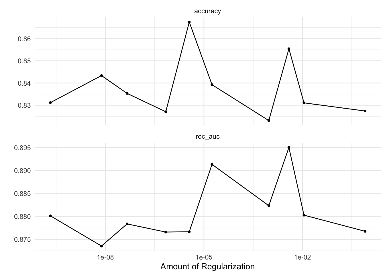
We can also use collect_metrics() to collect the results of tuning.
collect_metrics(logistic_reg_brulee_wf, summarize = TRUE)# A tibble: 20 × 7
penalty .metric .estimator mean n std_err .config
<dbl> <chr> <chr> <dbl> <int> <dbl> <chr>
1 1.11e- 2 accuracy binary 0.831 3 0.0257 Preprocessor1_Model01
2 1.11e- 2 roc_auc binary 0.880 3 0.00871 Preprocessor1_Model01
3 4.58e- 8 accuracy binary 0.835 3 0.00419 Preprocessor1_Model02
4 4.58e- 8 roc_auc binary 0.878 3 0.00766 Preprocessor1_Model02
5 7.60e- 9 accuracy binary 0.843 3 0.0121 Preprocessor1_Model03
6 7.60e- 9 roc_auc binary 0.874 3 0.00235 Preprocessor1_Model03
7 3.85e- 3 accuracy binary 0.855 3 0.0183 Preprocessor1_Model04
8 3.85e- 3 roc_auc binary 0.895 3 0.00220 Preprocessor1_Model04
9 1.76e- 5 accuracy binary 0.839 3 0.0115 Preprocessor1_Model05
10 1.76e- 5 roc_auc binary 0.891 3 0.00872 Preprocessor1_Model05
11 6.88e- 7 accuracy binary 0.827 3 0.0187 Preprocessor1_Model06
12 6.88e- 7 roc_auc binary 0.877 3 0.0192 Preprocessor1_Model06
13 3.57e- 6 accuracy binary 0.868 3 0.0182 Preprocessor1_Model07
14 3.57e- 6 roc_auc binary 0.877 3 0.00511 Preprocessor1_Model07
15 2.11e-10 accuracy binary 0.831 3 0.0130 Preprocessor1_Model08
16 2.11e-10 roc_auc binary 0.880 3 0.00217 Preprocessor1_Model08
17 8.03e- 1 accuracy binary 0.827 3 0.00706 Preprocessor1_Model09
18 8.03e- 1 roc_auc binary 0.877 3 0.0115 Preprocessor1_Model09
19 9.42e- 4 accuracy binary 0.823 3 0.0250 Preprocessor1_Model10
20 9.42e- 4 roc_auc binary 0.882 3 0.00516 Preprocessor1_Model10From the fitted workflow we can select the best model with the tune::select_best() function and the roc_auc metric. This metric is used to measure the ability of the model to distinguish between two classes, and is calculated by plotting the true positive rate against the false positive rate.
Once we’ve identified the best model, we can extract it from the workflow using the extract_workflow function. This function allows us to isolate the model and use it for further analysis. We then use the finalize_workflow function to finalize the model, and the last_fit function to fit the model to the ad_split data.
We use the collect_metrics function to gather metrics for the best model. This is an important step, as it allows us to evaluate the performance of the model and determine whether it is accurate and reliable.
Finally, we use the collect_predictions function to generate predictions on the test set, and use these predictions to create an ROC curve.
Select Best Logistic Regression Model and Evaluate
# select the best model from the workflow
best_logistic_reg_id <-
  logistic_reg_brulee_wf |>
  select_best(metric = "roc_auc")

# extract the best model from the workflow
best_logistic_reg <-
  logistic_reg_brulee_wf |>
  extract_workflow() |>
  finalize_workflow(best_logistic_reg_id) |>
  last_fit(ad_split)

# collect the metrics for the best model
best_logistic_reg |>
  collect_metrics()
# A tibble: 2 × 4
.metric .estimator .estimate .config
<chr> <chr> <dbl> <chr>
1 accuracy binary 0.833 Preprocessor1_Model1
2 roc_auc binary 0.865 Preprocessor1_Model1# plot results of test set fit
best_logistic_reg |>
collect_predictions() |>
roc_curve(Class, .pred_Impaired) |>
autoplot()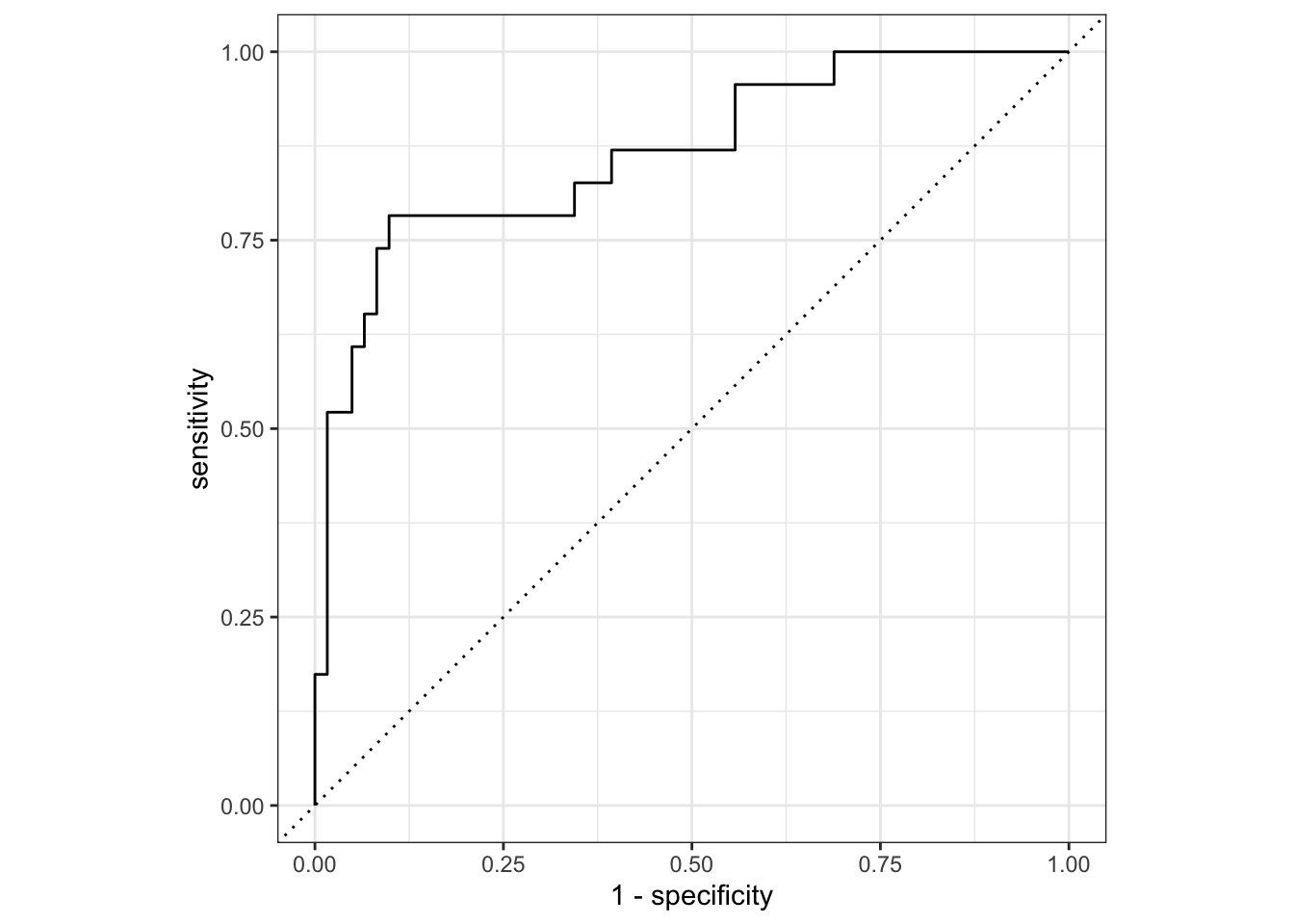
We start by fitting the workflow with the grid of hyperparameter values we created above. This will give us a starting point for Bayesian optimization.
Create MLP Workflow and Perform Grid Tuning
mlp_brulee_wf <-
  workflow() |>
  add_recipe(ad_rec) |>
  add_model(mlp_brulee_spec)

mlp_brulee_tune_grid <-
  mlp_brulee_wf |>
  tune_grid(
    resamples = ad_folds,
    grid      = mlp_brulee_start,
    control   = grid_control
  )
As above, autoplot() is a quick way to visualize results form our initial grid tuning.
autoplot(mlp_brulee_tune_grid)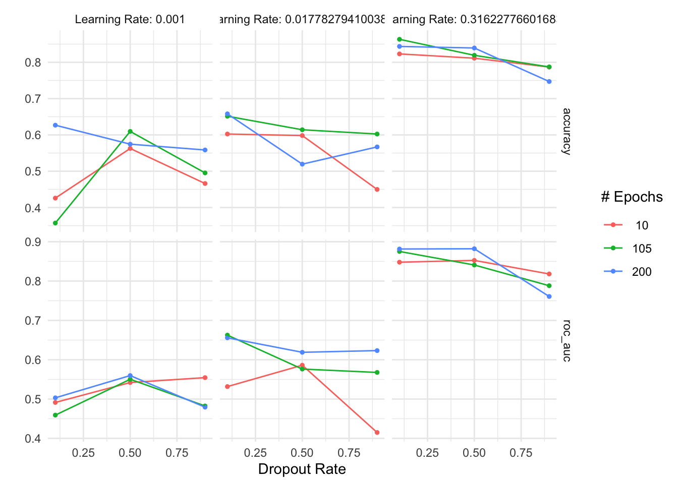
We can also repeat the best model selection and evaluation, as we did for logistic regression. Our expectation should be that Bayesian optimization results in better predictions that a simple tune_grid() approach.
Visualize and Evaluate Initial Tuning
best_mlp_id_no_bayes <-
  mlp_brulee_tune_grid |>
  select_best(metric = "roc_auc")

# extract the best model from the workflow
best_mlp_no_bayes <-
  mlp_brulee_tune_grid |>
  extract_workflow() |>
  finalize_workflow(best_mlp_id_no_bayes) |>
  last_fit(ad_split)

# collect the metrics for the best model
best_mlp_no_bayes |>
  collect_metrics()
# A tibble: 2 × 4
.metric .estimator .estimate .config
<chr> <chr> <dbl> <chr>
1 accuracy binary 0.833 Preprocessor1_Model1
2 roc_auc binary 0.852 Preprocessor1_Model1# plot results of test set fit
best_mlp_no_bayes |>
collect_predictions() |>
roc_curve(Class, .pred_Impaired) |>
autoplot()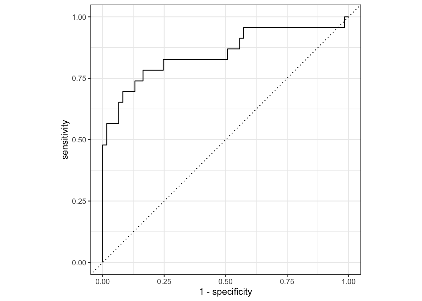
We now take the initial MLP tune results and pass them to tune_bayes(), which includes the initial grid of hyperparameter values, the folds we created above, and the bayes_control variables we created earlier.
Bayesian Optimization of MLP
mlp_brulee_bo <-
  mlp_brulee_wf |>
  tune_bayes(
    resamples = ad_folds,
    iter      = 100L,
    control   = bayes_control,
    initial   = mlp_brulee_tune_grid
  )
Optimizing roc_auc using the expected improvement! No improvement for 30 iterations; returning current results.Yet again, we can use autoplot() to visualize the results of tuning. From this, it appears that learning rate has a big impact on model performance, but number of epochs and droput rate are less important. Digging into why is beyond the scope of this post, but it’s important to recognize that not all hyperparameter are created equal.
autoplot(mlp_brulee_bo)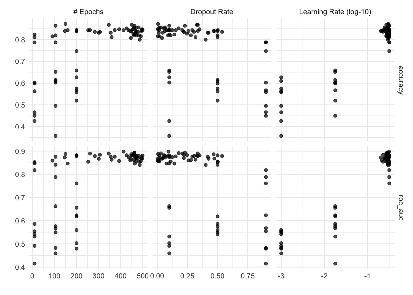
And yet again, we can use collect_metrics() to collect the results of tuning.
collect_metrics(mlp_brulee_bo, summarize = TRUE)# A tibble: 142 × 10
dropout epochs learn_rate .metric .estim…¹ mean n std_err .config .iter
<dbl> <int> <dbl> <chr> <chr> <dbl> <int> <dbl> <chr> <int>
1 0.1 10 0.001 accuracy binary 0.426 3 0.0897 Prepro… 0
2 0.1 10 0.001 roc_auc binary 0.491 3 0.0212 Prepro… 0
3 0.5 10 0.001 accuracy binary 0.563 3 0.111 Prepro… 0
4 0.5 10 0.001 roc_auc binary 0.542 3 0.0360 Prepro… 0
5 0.9 10 0.001 accuracy binary 0.466 3 0.0362 Prepro… 0
6 0.9 10 0.001 roc_auc binary 0.554 3 0.0576 Prepro… 0
7 0.1 105 0.001 accuracy binary 0.357 3 0.0274 Prepro… 0
8 0.1 105 0.001 roc_auc binary 0.459 3 0.0476 Prepro… 0
9 0.5 105 0.001 accuracy binary 0.610 3 0.0619 Prepro… 0
10 0.5 105 0.001 roc_auc binary 0.550 3 0.0707 Prepro… 0
# … with 132 more rows, and abbreviated variable name ¹.estimatorFor our moment of truth, we can select the best model and evaluate it on the test set.
Finalize Model and Evaluate
best_mlp_id <-
  mlp_brulee_bo |>
  select_best(metric = "roc_auc")

# extract the best model from the workflow
best_mlp <-
  mlp_brulee_bo |>
  extract_workflow() |>
  finalize_workflow(best_mlp_id) |>
  last_fit(ad_split)

# collect the metrics for the best model
best_mlp |>
  collect_metrics()
# A tibble: 2 × 4
.metric .estimator .estimate .config
<chr> <chr> <dbl> <chr>
1 accuracy binary 0.893 Preprocessor1_Model1
2 roc_auc binary 0.890 Preprocessor1_Model1# plot results of test set fit
best_mlp |>
collect_predictions() |>
roc_curve(Class, .pred_Impaired) |>
autoplot()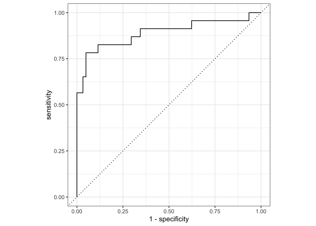
Based on these results, there was not much value in the Bayesian optimization in this case. Nonetheless, it is a useful tool to have in your toolbox, and I hope you find this example useful.